Model Building

Load packages and import datasets.

# load packages and basic settings
library(tidyverse)
library(modelr)
library(purrr)
library(MASS)

set.seed(1)

knitr::opts_chunk$set(
  fig.width = 6,
  fig.asp = .6,
  out.width = "90%"
)

theme_set(theme_minimal() + theme(legend.position = "bottom"))

options(
  ggplot2.continuous.colour = "viridis",
  ggplot2.continuous.fill = "viridis"
)

scale_colour_discrete = scale_colour_viridis_d
scale_fill_discrete = scale_fill_viridis_d

# import data (currently: using direct path)

# total cholesterol < 200 -> 0, >= 200 -> 1
model_df = read_csv("data/combine.csv") |> 
  mutate(
    chol_cat = ifelse(total_cholesterol < 200, 0, 1),
    alcohol_use_order = as.factor(alcohol_use_order),
    physical_activity = relevel(as.factor(physical_activity), ref = "Light/Unknown activity")
  )

# create subset for cholestorl level of desirable level and of above desirable level 
desire_df = 
  model_df |> 
  filter(chol_cat == 0)

ab_desire_df = 
  model_df |> 
  filter(chol_cat == 1)

Variables features

Continuous variables

Methods

For continuous variables, we use mean and standard deviation (std) to describe the distribution in overall samples, samples of desirable cholesterol level (defined as “control”), and samples of above-desirable cholesterol level (defined as “case”). Then, we use t-test to examine whether the means of these variables are significantly different between case group and control group (significance level = 0.05).

# mean and std for continuous variables, overall
list_conti_all = list(
  age = model_df$age, 
  bmi = model_df$bmi, 
  sleep_hour = model_df$sleep_hour, 
  cotinine = model_df$cotinine,
  chol_cat = model_df$chol_cat
) |> 
  as.data.frame()

list_conti_all_clean = 
  list_conti_all[-5] |> 
  lapply(na.omit)

mean_all = sapply(list_conti_all_clean, mean) |> 
  as.data.frame() |> 
  rename(overall_mean = "sapply(list_conti_all_clean, mean)")

std_all = sapply(list_conti_all_clean, sd) |> 
  as.data.frame() |> 
  rename(overall_std = "sapply(list_conti_all_clean, sd)")

# p-value of t test for continuous variables
t_test = function(variable) {
  t_test_result = t.test(list_conti_all[[variable]] ~ list_conti_all$chol_cat)
  return(data.frame(
    variable = variable,
    p_value = t_test_result$p.value
  ))
}

p_value = 
  lapply(c("age", "bmi", "sleep_hour", "cotinine"), t_test) |>
  bind_rows() |> 
  as.data.frame()

# mean and std for all continuous variables, among samples of desirable cholesteral level (named them as "control")
list_conti_desire = list(
  age = desire_df$age, 
  bmi = desire_df$bmi, 
  sleep_hour = desire_df$sleep_hour, 
  cotinine = desire_df$cotinine
) |> 
  as.data.frame() |> 
  lapply(na.omit)

mean_desire = sapply(list_conti_desire, mean) |> 
  as.data.frame() |> 
  rename(control_mean = "sapply(list_conti_desire, mean)")

std_desire = sapply(list_conti_desire, sd) |> 
  as.data.frame() |> 
  rename(control_std = "sapply(list_conti_desire, sd)")

# mean and std for all continuous variables, among samples of above-desirable cholesterol level (named them as "case")
list_conti_ab_desire = list(
  age = ab_desire_df$age, 
  bmi = ab_desire_df$bmi, 
  sleep_hour = ab_desire_df$sleep_hour, 
  cotinine = ab_desire_df$cotinine
) |> 
  as.data.frame() |> 
  lapply(na.omit)

mean_ab_desire = sapply(list_conti_ab_desire, mean) |> 
  as.data.frame() |> 
  rename(case_mean = "sapply(list_conti_ab_desire, mean)")

std_ab_desire = sapply(list_conti_ab_desire, sd) |> 
  as.data.frame() |> 
  rename(case_std = "sapply(list_conti_ab_desire, sd)")

Description table

# combind - continuous
conti_des_df =
  as.data.frame(cbind(mean_all, std_all, mean_desire, std_desire, mean_ab_desire, std_ab_desire, p_value))

conti_des_df = conti_des_df[, -grep("variable", colnames(conti_des_df))] |> 
  knitr::kable(digits = 3)

conti_des_df

	overall_mean	overall_std	control_mean	control_std	case_mean	case_std	p_value
age	49.414	18.302	48.014	19.312	52.326	15.604	0.000
bmi	29.914	7.536	29.993	7.870	29.750	6.787	0.150
sleep_hour	7.593	1.667	7.616	1.692	7.546	1.612	0.072
cotinine	55.683	128.581	57.823	131.881	51.232	121.334	0.026

• Based on the result, we can find that the age and cotinine is significantly different between case and control.

Binary and categorical variables

Methods

For binary and categorical variables, we use count (n) and percentage (pct) to describe the distribution in overall samples, samples of desirable cholesterol level (defined as “control”), and samples of above-desirable cholesterol level (defined as “case”). Then, as the data meet the assumption, we use chi-sq test to examine whether the distribution of these variables are significantly different between case group and control group (significance level = 0.05).

# n and pct for categorical variables, chi-sq test, overall
list_cat_all = list (
  gender = model_df$gender,
  race = model_df$race,
  marital = model_df$marital_status,
  edu = model_df$education_level_20,
  poverty = model_df$poverty_level,
  phy = model_df$physical_activity,
  alcohol = model_df$alcohol_use_cat,
  chol_cat = model_df$chol_cat
) |> 
  as.data.frame()

list_cat_all_clean = 
  list_cat_all[-8] |> 
  lapply(na.omit)

cat_vars = names(list_cat_all_clean)

count_all_function = function(variable) {
  table_value = table(list_cat_all[[variable]], list_cat_all$chol_cat)
  chi_sq_test = chisq.test(table_value)
  
  count = sapply(unique(list_cat_all_clean[[variable]], na.rm = TRUE), function(cat) sum(list_cat_all_clean[[variable]] == cat, na.rm = TRUE))
   
  total = sum(count)
  pct = count / total
  
  result_df = tibble(
    variable = names(count),
    n = count,
    pct = pct,
    p_value = chi_sq_test$p.value
    )
  
  return(result_df)
  }

cat_count_chisq = lapply(cat_vars, count_all_function) |> 
  bind_rows() |> 
  as.data.frame()

# n and pct for categorical variables, among samples of desirable cholesteral level (named them as "control")
list_cat_ctrl = list (
  gender = desire_df$gender,
  race = desire_df$race,
  marital = desire_df$marital_status,
  edu = desire_df$education_level_20,
  poverty = desire_df$poverty_level,
  phy = desire_df$physical_activity,
  alcohol = desire_df$alcohol_use_cat
) |> 
  as.data.frame() |> 
  lapply(na.omit)

cat_vars_ctrl = names(list_cat_ctrl)

count_ctrl_function = function(variable) {
  count = sapply(unique(list_cat_ctrl[[variable]], na.rm = TRUE), function(cat) sum(list_cat_ctrl[[variable]] == cat, na.rm = TRUE))
   
  total = sum(count)
  pct = count / total
  
  result_df = tibble(
    variable = names(count),
    control_n = count,
    control_pct = pct
    )
  
  return(result_df)
}

cat_count_ctrl = lapply(cat_vars_ctrl, count_ctrl_function) |> 
  bind_rows() |> 
  as.data.frame()

# n and pct for categorical variables, among samples of above-desirable cholesterol level (named them as "case")
list_cat_case = list (
  gender = ab_desire_df$gender,
  race = ab_desire_df$race,
  marital = ab_desire_df$marital_status,
  edu = ab_desire_df$education_level_20,
  poverty = ab_desire_df$poverty_level,
  phy = ab_desire_df$physical_activity,
  alcohol = ab_desire_df$alcohol_use_cat
) |> 
  as.data.frame() |> 
  lapply(na.omit)

cat_vars_case = names(list_cat_case)

count_case_function = function(variable) {
  count = sapply(unique(list_cat_case[[variable]], na.rm = TRUE), function(cat) sum(list_cat_case[[variable]] == cat, na.rm = TRUE))
   
  total = sum(count)
  pct = count / total
  
  result_df = tibble(
    variable = names(count),
    case_n = count,
    case_pct = pct
    )
  
  return(result_df)
}

cat_count_case = lapply(cat_vars_case, count_case_function) |> 
  bind_rows() |> 
  as.data.frame()

Description table

cat_des_df =
  cbind.data.frame(cat_count_chisq, cat_count_ctrl, cat_count_case) |> 
  drop_na()

cat_des_df = cat_des_df[, !duplicated(names(cat_des_df))] |> 
  knitr::kable(digits = 3)

cat_des_df

variable	n	pct	p_value	control_n	control_pct	case_n	case_pct
Female	4199	0.515	0.000	2725	0.494	1176	0.444
Male	3962	0.485	0.000	2786	0.506	1474	0.556
Non-Hispanic Asian	977	0.120	0.000	597	0.108	963	0.363
Non-Hispanic White	2878	0.353	0.000	1915	0.347	607	0.229
Other Race	396	0.049	0.000	260	0.047	380	0.143
Hispanic	1855	0.227	0.000	1491	0.271	564	0.213
Non-Hispanic Black	2055	0.252	0.000	1248	0.226	136	0.051
Never married	1497	0.192	0.000	1132	0.219	1601	0.613
Married/Living with Partner	4549	0.584	0.000	1093	0.211	365	0.140
Widowed/Divorced/Separated	1740	0.223	0.000	2948	0.570	647	0.248
College graduate or above	1919	0.247	0.005	1218	0.236	701	0.268
9-11th grade	850	0.109	0.005	571	0.110	279	0.107
Some college or AA degree	2551	0.328	0.005	1694	0.328	202	0.077
High school graduate/GED or equivalent	1873	0.241	0.005	1298	0.251	857	0.328
Less than 9th grade	591	0.076	0.005	389	0.075	575	0.220
Above 185% of Poverty Guidelines	3388	0.525	0.000	2209	0.509	1179	0.557
Below 130% of Poverty Guidelines	2085	0.323	0.000	1472	0.339	613	0.290
Between 130% and 185% of Poverty Guidelines	986	0.153	0.000	661	0.152	325	0.154
Light Drinker	3424	0.493	0.000	2378	0.507	1046	0.462
Moderate Drinker	2573	0.370	0.000	1736	0.370	837	0.370
Heavy Drinker	955	0.137	0.000	573	0.122	382	0.169

• Based on the result, we can find that all the binary and categorical variables are significantly different between case and control.

Building model

In this study, our response variable is total cholesterol level (total_cholesterol), and our explanatory variables are (1) cotinine (cotinine), (2) physical activity (physical_activity), and (3) alcohol use (alcohol_use_cat). Sleep_hour is not significantly different between total cholesterol of desirable level and of above desirable level, so we remove this variable for the next model building steps. We decide to analyze the association step by step (significance level = 0.05).

Check the dataset

model_df |> 
  ggplot(aes(x = cotinine, y = total_cholesterol)) + geom_point() +
  labs(title = "Total_cholesterol against Serum Cotinine", x = "Serum Cotinine (ng/ml)", y = "Total Cholesterol (mg/dL)")

model_df |> 
  ggplot(aes(x = alcohol_use_cat, y = total_cholesterol)) + geom_point() +
  labs(title = "Total_cholesterol against Alcohol Use", x = "Alcohol Use", y = "Total Cholesterol (mg/dL)")

model_df |> 
  ggplot(aes(x = physical_activity, y = total_cholesterol)) + geom_point() +
  labs(title = "Total_cholesterol against Physical_activity", x = "Physical Activity", y = "Total Cholesterol (mg/dL)")

model_df |> 
  ggplot(aes(x = total_cholesterol)) + geom_density() +
  labs(title = "Destribution of Total_cholesterol", x = "Total Cholesterol (mg/dL)")

• Based on the scatterplot, we can find slightly negative linear trends, but there is heteroscedasticity problem. Also, based on the density plot, we can find that the distribution of response variable (y) total_cholesterol is asymmetry. Therefore, we decide to use linear regression model with log-transformation on y for the following models.

Model selection

Here, we use seven ways to build up different models. For the first four models, we build them based on epidemiological views. For the sixth, seventh, and eighth models, we build them based on biostatistical knowledge (AIC value, backward selection, and stepwise selection) combined with epidemiological views.

1. main explanatory variable: cotinine

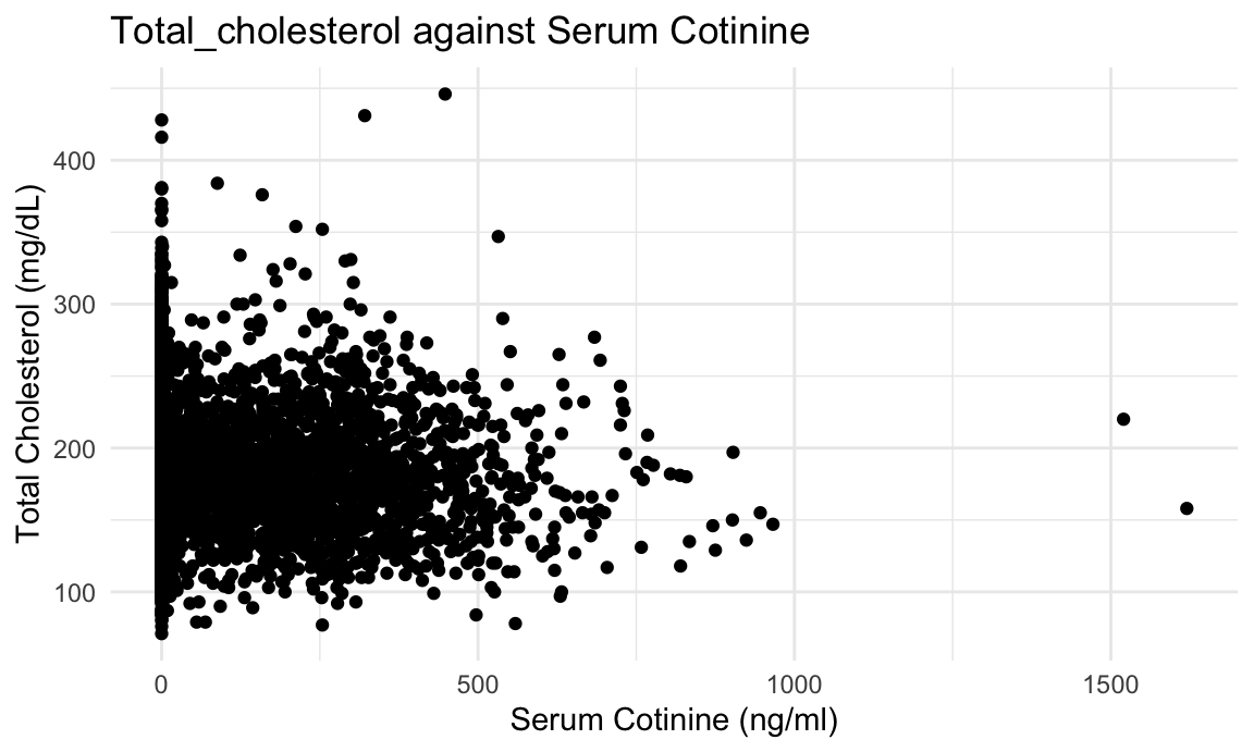
We hypothesize that cotinine, an indicator of exposure of smoking, is positively associated with the log of total cholesterol.

1) Univariable linear regression

fit_1: log(total_cholesterol) = cotinine

fit_1 = lm(log(total_cholesterol) ~ cotinine, data = model_df)

fit_1 |> 
  broom::tidy() |> 
  knitr::kable(digits = 3)

term	estimate	std.error	statistic	p.value
(Intercept)	5.198	0.003	1944.859	0
cotinine	0.000	0.000	-3.776	0

model_df |> 
  modelr::add_residuals(fit_1) |> 
  ggplot(aes(sample = resid)) +
  stat_qq() +
  stat_qq_line() +
  labs(title = "QQ Plot", x = "Quantile", y = "Residual")

• We can see that cotinine is significantly associated with total cholesterol level. We also check the qq-plot and find that the residuals followed a normal distribution, which indicates a suitability of using linear regression.
• Therefore, we move forward to build multivariable regression.

2) Multivariable linear regression

fit_cot: log(total_cholesterol) = cotinine + age + gender + race + marital_status + education_level_20 + poverty_level

fit_cot = lm(log(total_cholesterol) ~ cotinine + age + gender + race + marital_status + education_level_20 + poverty_level, data = model_df)

fit_cot |> 
  broom::tidy() |> 
  knitr::kable(digits = 3)

term	estimate	std.error	statistic	p.value
(Intercept)	5.221	0.015	354.487	0.000
cotinine	0.000	0.000	-0.192	0.847
age	0.000	0.000	1.297	0.195
genderMale	-0.045	0.006	-7.911	0.000
raceNon-Hispanic Asian	0.013	0.011	1.186	0.236
raceNon-Hispanic Black	-0.034	0.009	-3.899	0.000
raceNon-Hispanic White	-0.012	0.008	-1.463	0.144
raceOther Race	0.009	0.014	0.607	0.544
marital_statusNever married	-0.039	0.008	-4.903	0.000
marital_statusWidowed/Divorced/Separated	0.011	0.007	1.442	0.149
education_level_20College graduate or above	0.026	0.011	2.361	0.018
education_level_20High school graduate/GED or equivalent	-0.005	0.010	-0.471	0.638
education_level_20Less than 9th grade	0.013	0.014	0.893	0.372
education_level_20Some college or AA degree	0.010	0.010	1.006	0.314
poverty_levelBelow 130% of Poverty Guidelines	-0.013	0.007	-1.811	0.070
poverty_levelBetween 130% and 185% of Poverty Guidelines	-0.002	0.008	-0.214	0.831

• Based on the estimates of alcohol_use_cat, we can see no association between cotinine and log total cholesterol. This is not consistent with our hypothesis, and the estimate is not significant at 0.05 level of significance.

2. main explanatory variable: physical_activity

We hypothesize that physical activity is negatively associated with the log of total cholesterol.

1) Univariable linear regression

fit_2: total_cholesterol = physical_activity

fit_2 = lm(log(total_cholesterol) ~ physical_activity, data = model_df)

fit_2 |> 
  broom::tidy() |> 
  knitr::kable(digits = 3)

term	estimate	std.error	statistic	p.value
(Intercept)	5.197	0.005	1039.540	0.000
physical_activityModerate activity	0.004	0.007	0.599	0.549
physical_activityVigorous activity	-0.010	0.006	-1.570	0.117

model_df |> 
  modelr::add_residuals(fit_2) |> 
  ggplot(aes(sample = resid)) +
  stat_qq() +
  stat_qq_line() +
  labs(title = "QQ Plot", x = "Quantile", y = "Residual")

• We can see that physical_activity is not significantly associated with total cholesterol level. We also check the qq-plot and find that the residuals followed a normal distribution, which indicates a suitability of using linear regression.
• Though no significant result found, we think maybe it is the confounders that conceal the association. Therefore, we move forward to build multivariable regression.

2) Multivariable linear regression

fit_phy: log(total_cholesterol) = physical_activity + age + gender + race + marital_status + education_level_20 + poverty_level

fit_phy = lm(log(total_cholesterol) ~ physical_activity + age + gender + race + marital_status + education_level_20 + poverty_level, data = model_df)

fit_phy |> 
  broom::tidy() |> 
  knitr::kable(digits = 3)

term	estimate	std.error	statistic	p.value
(Intercept)	5.212	0.016	323.926	0.000
physical_activityModerate activity	0.006	0.007	0.773	0.439
physical_activityVigorous activity	0.010	0.008	1.278	0.201
age	0.000	0.000	1.608	0.108
genderMale	-0.047	0.006	-8.062	0.000
raceNon-Hispanic Asian	0.013	0.011	1.229	0.219
raceNon-Hispanic Black	-0.034	0.009	-3.937	0.000
raceNon-Hispanic White	-0.012	0.008	-1.524	0.128
raceOther Race	0.008	0.014	0.528	0.597
marital_statusNever married	-0.039	0.008	-4.897	0.000
marital_statusWidowed/Divorced/Separated	0.010	0.007	1.409	0.159
education_level_20College graduate or above	0.025	0.011	2.315	0.021
education_level_20High school graduate/GED or equivalent	-0.005	0.010	-0.515	0.607
education_level_20Less than 9th grade	0.013	0.014	0.909	0.364
education_level_20Some college or AA degree	0.010	0.010	0.971	0.332
poverty_levelBelow 130% of Poverty Guidelines	-0.012	0.007	-1.731	0.083
poverty_levelBetween 130% and 185% of Poverty Guidelines	-0.001	0.008	-0.150	0.881

• Based on the estimates of alcohol_use_cat, we can see that compared to population with light activity (reference group), population with moderate activity and vigorous activity both have higher total cholesterol. This is not consistent with our hypothesis, and the association is not significant at 0.05 level of significance.

3. main explanatory variable: alcohol_use_cat

We hypothesize that alcohol drinking is positively associated with the log of total cholesterol.

1) Univariable linear regression

fit_3: total_cholesterol = alcohol_use_cat

fit_3 = lm(log(total_cholesterol) ~ alcohol_use_cat, data = model_df)

fit_3 |> 
  broom::tidy() |> 
  knitr::kable(digits = 3)

term	estimate	std.error	statistic	p.value
(Intercept)	5.235	0.007	729.265	0
alcohol_use_catLight Drinker	-0.054	0.008	-6.703	0
alcohol_use_catModerate Drinker	-0.040	0.008	-4.732	0

model_df |> 
  modelr::add_residuals(fit_3) |> 
  ggplot(aes(sample = resid)) +
  stat_qq() +
  stat_qq_line() +
  labs(title = "QQ Plot", x = "Quantile", y = "Residual")

• We can see that alcohol_use_cat is significantly positively associated with total cholesterol level. We also check the qq-plot and find that the residuals followed a normal distribution, which indicates a suitability of using linear regression.
• Therefore, we move forward to build multivariable regression.

2) Multivariable linear regression

fit_alc: log(total_cholesterol) = alcohol_use_cat + age + gender + race + marital_status + education_level_20 + poverty_level

fit_alc = lm(log(total_cholesterol) ~ alcohol_use_cat + age + gender + race + marital_status + education_level_20 + poverty_level, data = model_df)

fit_alc |> 
  broom::tidy() |> 
  knitr::kable(digits = 3)

term	estimate	std.error	statistic	p.value
(Intercept)	5.281	0.018	296.615	0.000
alcohol_use_catLight Drinker	-0.066	0.009	-7.277	0.000
alcohol_use_catModerate Drinker	-0.046	0.009	-4.884	0.000
age	0.000	0.000	1.045	0.296
genderMale	-0.056	0.006	-9.141	0.000
raceNon-Hispanic Asian	0.019	0.013	1.516	0.130
raceNon-Hispanic Black	-0.038	0.009	-4.099	0.000
raceNon-Hispanic White	-0.015	0.009	-1.734	0.083
raceOther Race	0.010	0.015	0.699	0.485
marital_statusNever married	-0.039	0.009	-4.587	0.000
marital_statusWidowed/Divorced/Separated	0.012	0.008	1.504	0.133
education_level_20College graduate or above	0.021	0.012	1.758	0.079
education_level_20High school graduate/GED or equivalent	-0.009	0.011	-0.815	0.415
education_level_20Less than 9th grade	0.031	0.017	1.852	0.064
education_level_20Some college or AA degree	0.008	0.011	0.730	0.465
poverty_levelBelow 130% of Poverty Guidelines	-0.014	0.008	-1.881	0.060
poverty_levelBetween 130% and 185% of Poverty Guidelines	0.002	0.009	0.277	0.782

• Based on the estimates of alcohol_use_cat, we can see that compared to heavy drinkers (reference group), light drinkers and moderate drinkers both have significant lower total cholesterol. Light drinkers have lower risk than moderate drinkers. This is consistent with our hypothesis

4. explanatory variables: cotinine, physical_activity, and alcohol_use_cat

We assume that smoking (implied by cotinine), alcohol drinking, and physical activity could be potentially related to each other. Therefrore, a full model including these three variables to adjust their influence to each other makes sense.

fit_full: log(total_cholesterol) = cotinine + physical_activity + alcohol_use_cat + age + gender + race + marital_status + education_level_20 + poverty_level

fit_full = lm(log(total_cholesterol) ~ cotinine + physical_activity + alcohol_use_cat + age + gender + race + marital_status + education_level_20 + poverty_level, data = model_df)

fit_full |> 
  broom::tidy() |> 
  knitr::kable(digits = 3)

term	estimate	std.error	statistic	p.value
(Intercept)	5.277	0.019	272.405	0.000
cotinine	0.000	0.000	-0.350	0.727
physical_activityModerate activity	0.007	0.008	0.822	0.411
physical_activityVigorous activity	0.006	0.008	0.686	0.493
alcohol_use_catLight Drinker	-0.066	0.009	-7.220	0.000
alcohol_use_catModerate Drinker	-0.046	0.009	-4.889	0.000
age	0.000	0.000	1.070	0.285
genderMale	-0.056	0.006	-8.936	0.000
raceNon-Hispanic Asian	0.019	0.013	1.510	0.131
raceNon-Hispanic Black	-0.038	0.009	-4.008	0.000
raceNon-Hispanic White	-0.015	0.009	-1.678	0.093
raceOther Race	0.011	0.015	0.718	0.473
marital_statusNever married	-0.040	0.009	-4.601	0.000
marital_statusWidowed/Divorced/Separated	0.012	0.008	1.532	0.126
education_level_20College graduate or above	0.020	0.012	1.648	0.100
education_level_20High school graduate/GED or equivalent	-0.010	0.011	-0.857	0.391
education_level_20Less than 9th grade	0.030	0.017	1.820	0.069
education_level_20Some college or AA degree	0.007	0.011	0.663	0.508
poverty_levelBelow 130% of Poverty Guidelines	-0.013	0.008	-1.778	0.075
poverty_levelBetween 130% and 185% of Poverty Guidelines	0.003	0.009	0.338	0.735

5. AIC value selection

fit_full = lm(log(total_cholesterol) ~ cotinine + physical_activity + alcohol_use_cat + age + gender + race + marital_status + education_level_20 + poverty_level, data = model_df)

test_aic = stepAIC(fit_full, direction = "both", trace = FALSE)

summary(test_aic)

## 
## Call:
## lm(formula = log(total_cholesterol) ~ alcohol_use_cat + gender + 
##     race + marital_status + education_level_20 + poverty_level, 
##     data = model_df)
## 
## Residuals:
##      Min       1Q   Median       3Q      Max 
## -0.98018 -0.14515  0.00187  0.14798  0.92464 
## 
## Coefficients:
##                                                           Estimate Std. Error
## (Intercept)                                               5.291661   0.014773
## alcohol_use_catLight Drinker                             -0.066035   0.009119
## alcohol_use_catModerate Drinker                          -0.046470   0.009319
## genderMale                                               -0.055600   0.006121
## raceNon-Hispanic Asian                                    0.019256   0.012542
## raceNon-Hispanic Black                                   -0.037329   0.009297
## raceNon-Hispanic White                                   -0.013509   0.008446
## raceOther Race                                            0.010565   0.014961
## marital_statusNever married                              -0.042028   0.008227
## marital_statusWidowed/Divorced/Separated                  0.013753   0.007551
## education_level_20College graduate or above               0.020305   0.011820
## education_level_20High school graduate/GED or equivalent -0.009487   0.011201
## education_level_20Less than 9th grade                     0.031655   0.016478
## education_level_20Some college or AA degree               0.007220   0.010858
## poverty_levelBelow 130% of Poverty Guidelines            -0.015045   0.007450
## poverty_levelBetween 130% and 185% of Poverty Guidelines  0.002317   0.008895
##                                                          t value Pr(>|t|)    
## (Intercept)                                              358.207  < 2e-16 ***
## alcohol_use_catLight Drinker                              -7.242 5.06e-13 ***
## alcohol_use_catModerate Drinker                           -4.987 6.33e-07 ***
## genderMale                                                -9.084  < 2e-16 ***
## raceNon-Hispanic Asian                                     1.535   0.1248    
## raceNon-Hispanic Black                                    -4.015 6.02e-05 ***
## raceNon-Hispanic White                                    -1.599   0.1098    
## raceOther Race                                             0.706   0.4801    
## marital_statusNever married                               -5.109 3.35e-07 ***
## marital_statusWidowed/Divorced/Separated                   1.821   0.0686 .  
## education_level_20College graduate or above                1.718   0.0859 .  
## education_level_20High school graduate/GED or equivalent  -0.847   0.3971    
## education_level_20Less than 9th grade                      1.921   0.0548 .  
## education_level_20Some college or AA degree                0.665   0.5061    
## poverty_levelBelow 130% of Poverty Guidelines             -2.019   0.0435 *  
## poverty_levelBetween 130% and 185% of Poverty Guidelines   0.260   0.7945    
## ---
## Signif. codes:  0 '***' 0.001 '**' 0.01 '*' 0.05 '.' 0.1 ' ' 1
## 
## Residual standard error: 0.2188 on 5393 degrees of freedom
##   (2752 observations deleted due to missingness)
## Multiple R-squared:  0.04106,    Adjusted R-squared:  0.0384 
## F-statistic:  15.4 on 15 and 5393 DF,  p-value: < 2.2e-16

• Based on the output, we can find the best model optimized by comparing AIC value is log(total_cholesterol) = alcohol_use_cat + gender + race + marital_status + education_level_20 + poverty_level. However, we think variable age is an essential variable when studying health outcome, such as total cholesterol in this study. Therefore, we decide to add variable age into this model, and summary the final model for comparing is log(total_cholesterol) = alcohol_use_cat + age + gender + race + marital_status + education_level_20 + poverty_level, which is the same as model fit_alc.

6. Backwawrd selection on full model

fit_backward = step(fit_full, direction = "backward")

## Start:  AIC=-16415.57
## log(total_cholesterol) ~ cotinine + physical_activity + alcohol_use_cat + 
##     age + gender + race + marital_status + education_level_20 + 
##     poverty_level
## 
##                      Df Sum of Sq    RSS    AIC
## - physical_activity   2    0.0350 258.19 -16419
## - cotinine            1    0.0059 258.16 -16417
## - age                 1    0.0548 258.21 -16416
## <none>                            258.16 -16416
## - poverty_level       2    0.2038 258.36 -16415
## - education_level_20  4    0.6827 258.84 -16409
## - marital_status      2    1.3044 259.46 -16392
## - race                4    1.5203 259.68 -16392
## - alcohol_use_cat     2    2.5173 260.67 -16367
## - gender              1    3.8255 261.98 -16338
## 
## Step:  AIC=-16418.83
## log(total_cholesterol) ~ cotinine + alcohol_use_cat + age + gender + 
##     race + marital_status + education_level_20 + poverty_level
## 
##                      Df Sum of Sq    RSS    AIC
## - cotinine            1    0.0067 258.20 -16421
## - age                 1    0.0485 258.24 -16420
## <none>                            258.19 -16419
## - poverty_level       2    0.2075 258.40 -16418
## - education_level_20  4    0.6884 258.88 -16412
## - marital_status      2    1.2950 259.49 -16396
## - race                4    1.5302 259.72 -16395
## - alcohol_use_cat     2    2.5655 260.76 -16369
## - gender              1    3.9007 262.09 -16340
## 
## Step:  AIC=-16420.69
## log(total_cholesterol) ~ alcohol_use_cat + age + gender + race + 
##     marital_status + education_level_20 + poverty_level
## 
##                      Df Sum of Sq    RSS    AIC
## - age                 1    0.0523 258.25 -16422
## <none>                            258.20 -16421
## - poverty_level       2    0.2172 258.42 -16420
## - education_level_20  4    0.7140 258.91 -16414
## - marital_status      2    1.2913 259.49 -16398
## - race                4    1.5580 259.75 -16396
## - alcohol_use_cat     2    2.5598 260.76 -16371
## - gender              1    4.0009 262.20 -16340
## 
## Step:  AIC=-16421.6
## log(total_cholesterol) ~ alcohol_use_cat + gender + race + marital_status + 
##     education_level_20 + poverty_level
## 
##                      Df Sum of Sq    RSS    AIC
## <none>                            258.25 -16422
## - poverty_level       2    0.2465 258.50 -16420
## - education_level_20  4    0.7266 258.98 -16414
## - race                4    1.5164 259.77 -16398
## - marital_status      2    1.8116 260.06 -16388
## - alcohol_use_cat     2    2.5279 260.78 -16373
## - gender              1    3.9513 262.20 -16342

• Based on the output, we can find the best model optimized by backward selection summary for full model with log transfermation on y is log(total_cholesterol) = alcohol_use_cat + gender + race + marital_status + education_level_20 + poverty_level. However, we think variable age is an essential variable when studying health outcome, such as total cholesterol in this study. Therefore, we decide to add variable age into this model, and summary the final model for comparing is log(total_cholesterol) = alcohol_use_cat + age + gender + race + marital_status + education_level_20 + poverty_level, which is the same as model fit_alc.

7. Stepwise selection on full model

fit_stepwise = step(fit_full)

## Start:  AIC=-16415.57
## log(total_cholesterol) ~ cotinine + physical_activity + alcohol_use_cat + 
##     age + gender + race + marital_status + education_level_20 + 
##     poverty_level
## 
##                      Df Sum of Sq    RSS    AIC
## - physical_activity   2    0.0350 258.19 -16419
## - cotinine            1    0.0059 258.16 -16417
## - age                 1    0.0548 258.21 -16416
## <none>                            258.16 -16416
## - poverty_level       2    0.2038 258.36 -16415
## - education_level_20  4    0.6827 258.84 -16409
## - marital_status      2    1.3044 259.46 -16392
## - race                4    1.5203 259.68 -16392
## - alcohol_use_cat     2    2.5173 260.67 -16367
## - gender              1    3.8255 261.98 -16338
## 
## Step:  AIC=-16418.83
## log(total_cholesterol) ~ cotinine + alcohol_use_cat + age + gender + 
##     race + marital_status + education_level_20 + poverty_level
## 
##                      Df Sum of Sq    RSS    AIC
## - cotinine            1    0.0067 258.20 -16421
## - age                 1    0.0485 258.24 -16420
## <none>                            258.19 -16419
## - poverty_level       2    0.2075 258.40 -16418
## - education_level_20  4    0.6884 258.88 -16412
## - marital_status      2    1.2950 259.49 -16396
## - race                4    1.5302 259.72 -16395
## - alcohol_use_cat     2    2.5655 260.76 -16369
## - gender              1    3.9007 262.09 -16340
## 
## Step:  AIC=-16420.69
## log(total_cholesterol) ~ alcohol_use_cat + age + gender + race + 
##     marital_status + education_level_20 + poverty_level
## 
##                      Df Sum of Sq    RSS    AIC
## - age                 1    0.0523 258.25 -16422
## <none>                            258.20 -16421
## - poverty_level       2    0.2172 258.42 -16420
## - education_level_20  4    0.7140 258.91 -16414
## - marital_status      2    1.2913 259.49 -16398
## - race                4    1.5580 259.75 -16396
## - alcohol_use_cat     2    2.5598 260.76 -16371
## - gender              1    4.0009 262.20 -16340
## 
## Step:  AIC=-16421.6
## log(total_cholesterol) ~ alcohol_use_cat + gender + race + marital_status + 
##     education_level_20 + poverty_level
## 
##                      Df Sum of Sq    RSS    AIC
## <none>                            258.25 -16422
## - poverty_level       2    0.2465 258.50 -16420
## - education_level_20  4    0.7266 258.98 -16414
## - race                4    1.5164 259.77 -16398
## - marital_status      2    1.8116 260.06 -16388
## - alcohol_use_cat     2    2.5279 260.78 -16373
## - gender              1    3.9513 262.20 -16342

• Based on the output, we can find the best model optimized by stepwise selection summary for full model with log transfermation on y is log(total_cholesterol) = alcohol_use_cat + gender + race + marital_status + education_level_20 + poverty_level. However, we think variable age is an essential variable when studying health outcome, such as total cholesterol in this study. Therefore, we decide to add variable age into this model, and summary the final model for comparing is log(total_cholesterol) = alcohol_use_cat + age + gender + race + marital_status + education_level_20 + poverty_level, which is the same as model fit_alc.

Model comparison

1. Cross validation

Based on the above steps, we now are comparing four models: fit_cot, fit_phy, fit_alc, and fit_full.

model_cv_df = 
  model_df |> 
  mutate(
    physical_activity = ifelse(physical_activity == "Light/Unknown activity", 0, ifelse(physical_activity == "Moderate activity", 1, 2)),
    alcohol_use_cat = ifelse(alcohol_use_cat == "Light Drinker", 0, ifelse(alcohol_use_cat == "Moderate Drinker", 1, 2))
    )

# create training and testing sets
cv_df =
  model_cv_df |> 
  crossv_mc(n = 300) |> 
  mutate(
    train = map(train, as_tibble),
    test = map(test, as_tibble)
  )

cv_results =
  cv_df |> 
  mutate(
    fit_cot = map(train, \(df) lm(log(total_cholesterol) ~ cotinine + age + gender + race + marital_status + education_level_20 + poverty_level, data = df)),
    fit_phy = map(train, \(df) lm(log(total_cholesterol) ~ physical_activity + age + gender + race + marital_status + education_level_20 + poverty_level, data = df)),
    fit_alc = map(train, \(df) lm(log(total_cholesterol) ~ alcohol_use_cat + age + gender + race + marital_status + education_level_20 + poverty_level, data = df)),
    fit_full = map(train, \(df) lm(log(total_cholesterol) ~ cotinine + physical_activity + alcohol_use_cat + age + gender + race + marital_status + education_level_20 + poverty_level, data = df))
  ) |> 
  mutate(
    rmse_fit_cot = map2_dbl(fit_cot, test, \(model, df) rmse(model, df)),
    rmse_fit_phy = map2_dbl(fit_phy, test, \(model, df) rmse(model, df)),
    rmse_fit_alc = map2_dbl(fit_alc, test, \(model, df) rmse(model, df)),
    rmse_fit_full = map2_dbl(fit_full, test, \(model, df) rmse(model, df))
  )

cv_results |> 
  dplyr::select(starts_with("rmse")) |> 
  pivot_longer(
    everything(),
    names_to = "model_type",
    values_to = "rmse",
    names_prefix = "rmse_"
  ) |> 
  ggplot(aes(x = model_type, y = rmse)) + geom_violin() +
  labs(x = "Model Type")

• Based on the violin plot, these four models have similar spread of root mean squared error.

2. r square

rsquare_fit_cot = rsquare(fit_cot, data = model_df)
rsquare_fit_phy = rsquare(fit_phy, data = model_df)
rsquare_fit_alc = rsquare(fit_alc, data = model_df)
rsquare_fit_full = rsquare(fit_full, data = model_df)

cbind(rsquare_fit_cot, rsquare_fit_phy, rsquare_fit_alc, rsquare_fit_full) |> 
  knitr::kable()

rsquare_fit_cot	rsquare_fit_phy	rsquare_fit_alc	rsquare_fit_full
0.0280454	0.0282958	0.0287445	0.0289015

• Based on the violin plot, these four models have similar r square values.

Conclusion

We decide to use model fit_alc: lm(log(total_cholesterol) = alcohol_use_cat + age + gender + race + marital_status + education_level_20 + poverty_level as our final model. With similar rmse distribution and r square, model fit_alc is less complex than model fit_full, and AIC value, backward selection, and stepwise selection all indicate this model is the best.

Take a deeper look at the estiamtes of model fit_alcs:

fit_alc |> 
  broom::tidy() |> 
  knitr::kable(digits = 3)

term	estimate	std.error	statistic	p.value
(Intercept)	5.281	0.018	296.615	0.000
alcohol_use_catLight Drinker	-0.066	0.009	-7.277	0.000
alcohol_use_catModerate Drinker	-0.046	0.009	-4.884	0.000
age	0.000	0.000	1.045	0.296
genderMale	-0.056	0.006	-9.141	0.000
raceNon-Hispanic Asian	0.019	0.013	1.516	0.130
raceNon-Hispanic Black	-0.038	0.009	-4.099	0.000
raceNon-Hispanic White	-0.015	0.009	-1.734	0.083
raceOther Race	0.010	0.015	0.699	0.485
marital_statusNever married	-0.039	0.009	-4.587	0.000
marital_statusWidowed/Divorced/Separated	0.012	0.008	1.504	0.133
education_level_20College graduate or above	0.021	0.012	1.758	0.079
education_level_20High school graduate/GED or equivalent	-0.009	0.011	-0.815	0.415
education_level_20Less than 9th grade	0.031	0.017	1.852	0.064
education_level_20Some college or AA degree	0.008	0.011	0.730	0.465
poverty_levelBelow 130% of Poverty Guidelines	-0.014	0.008	-1.881	0.060
poverty_levelBetween 130% and 185% of Poverty Guidelines	0.002	0.009	0.277	0.782

• Compared to heavy drinkers (reference group), light drinkers would have 0.066mg/dL less log(total_cholesterol) and moderate drinkers would have 0.046mg/dL less log(total_cholesterol), adjusting for age, gender, race, marital status, education level, and poverty level, based on this sample. This association is significant at 0.05 level of significance.

Then, We save this model as a RDS file for the next part: Predict Your Risk.

save_path = "fit_alc.rds"
saveRDS(fit_alc, save_path)